In the master’s courses on Control Systems at the Eindhoven University of Technology, we learn about amazing techniques for feedback and feedforward control.
However, we’re usually given a ready-to-use Matlab/Simulink environment, set up on an ancient real-time Linux kernel with EtherCAT, achieving sample rates of 2-4 kHz. I wanted to play around with control systems at home and such a setup was too expensive, slow, and cumbersome for my liking.
So instead, I decided to set up a hard real-time platform for less than €10 worth of hardware, capable of reaching at least 8 kHz sample rates. The application: closed-loop control of an old A4 consumer printer. The main goal is to implement Iterative Learning Control (ILC) on this printer, and possibly LQG and direct data-driven control.
In this blog, I’ll write updates on my progress. The audience I’m writing for is people who have a decent understanding of control systems, but want to learn more about the (low-cost) application to real systems. For those unfamiliar with control systems, this paper is a great place to start. My own specialization is Learning Control, and I’m a beginner in electronics and embedded systems. Expect cool control techniques and poor soldering jobs. I appreciate any feedback in the comments, especially about embedded systems and electronics.
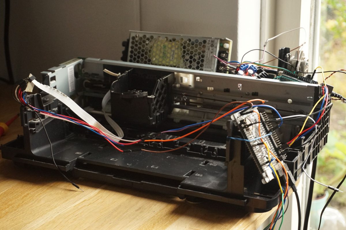
The printer while I’m still prototyping
This blog series will be structured as follows:
Part 1: Requirements, Preferences and Constraints. Here, I’ll outline the exact specifications I set at the start.
Part 2: Hardware selection, in which I compare several options and explain why I ended up buying these specific parts.
Part 3: Initial design of the real-time platform. In this part, I describe how I achieve a hard real-time control loop and how the printer communicates with my computer without loss of samples.
Part 4: Modeling and controller design. I’ll perform a Frequency Response Function (FRF) measurement and fit a transfer function. A feedback controller is designed in this part too.
Part 5: Implementation of Iterative Learning Control, and comparison of the performance with basic feedforward.
Part 6: On implementation aspects of control, where I explain what I learned about the practical side of control engineering.
A sneak preview of the results:
Tracking error for different iterations of ILC. The error is reduced significantly after 20 iterations.
Don’t hesitate to leave comments if you have questions/suggestions or if you learned something, I’m happy to respond! Start reading here.
In this blog post, I’ll outline the requirements, preferences and constraints for the project.
Requirements
1. The sample rate must be larger than 8 kHz. Why? Because I intend to use this real-time platform for all future projects that I might think of, and since some of those may involve very high stiffness. With the high-frequent resonant dynamics that come with such a system, having a relatively low sample time would introduce phase-lag in frequency regions where I’d be trying to get performance. For this project, 1 kHz would probably suffice, but I’ll go as high as I can with the hardware I get.
2. The control loop must be hard real-time. Whatever method I end up choosing to run the real-time loop, the sample time must remain constant over an experiment. I want to rely heavily on linear control theory, and this only makes sense for constant sample times.
3. Data logging must keep up with the sample rate, without dropping samples. At 8 kHz, and two 16-bit integers per sample, this is about 256 kBit/s.
4.The PWM resolution must be at least 12 bit. The PWM resolution indicates the number of different duty-cycles it can take on. Since the motor of my printer takes at most 24V, 12 bits corresponds to a 5 mV resolution. That sounds good enough to me.
5. The PWM frequency must keep up with the sample rate. If the PWM frequency is larger than the sample rate, it can not complete a full period with some duty cycle before the next sample determines a new duty cycle. Let’s say that one sample must include at least two full PWM periods, to be safe. Then the PWM frequency must be at least 16 kHz. Since fPWM = fclock / 2bits_resolution (see the previous link), I need a microcontroller with a PWM-enabled hardware timer with a resolution of >12 bits and a corresponding timer clock speed of >65 Mhz.
Preferences
1. The workflow should be user-friendly. I’m fine with programming in C, instead of working in Simulink. However, if possible, I don’t want to need to write software in assembly to achieve the required performance.
2. The print-head should move as precisely and fast as possible. I’m not sure yet where to put the trade-off between precision and speed, but when I have more feeling for what is physically possible, I’ll see if I can increase the print-speed while remaining the original print resolution (not that it can still print).
3. The real-time platform must be easily extendable to different projects. My next project is likely going to be a high-speed plotter, laser-engraver or laser cutter. I want my work here to be easily applicable there.
Constraints
Since I don’t want to change any of the printer hardware (at least the driveline), I must work with what I’ve got, which poses the following constraints.
1. I must work with a 24V brushed DC motor and position measurements, coming from a photo-interrupter and a strip of about 8000 slits over 30 cm. So the measurement resolution is about 38 μm. Printers like this that I find online typically draw at most 20W, so the power supply and motor driver need to tolerate about 1A.
2. The budget for the real-time platform is €10, for printer hardware it’s €30. It’s a hobby. It doesn’t need to be expensive. For printer hardware, the power supply takes up about €20. I might have used the original power supply, but in this case I prefer the freedom this gives me.
If I forgot anything, I’ll add it later. The next post will cover how I selected the parts based on these requirements.
With the requirements, preferences and constraints defined, let’s choose the hardware.
Microcontroller
Let’s start with the most common choices that people make for hobby projects: Arduino or Raspberry Pi. Neither of these are suitable here. Arduinos have at most PWM frequencies of 1000 Hz and 12 bit resolution, which is far lower than the 16 kHz I required in the previous post. Raspberry Pi might have the required specs, I’m not too sure, but it costs much more than the budgeted €10 and would involve setting up a real-time kernel. For these two reasons I’m crossing the Pi off the list too.
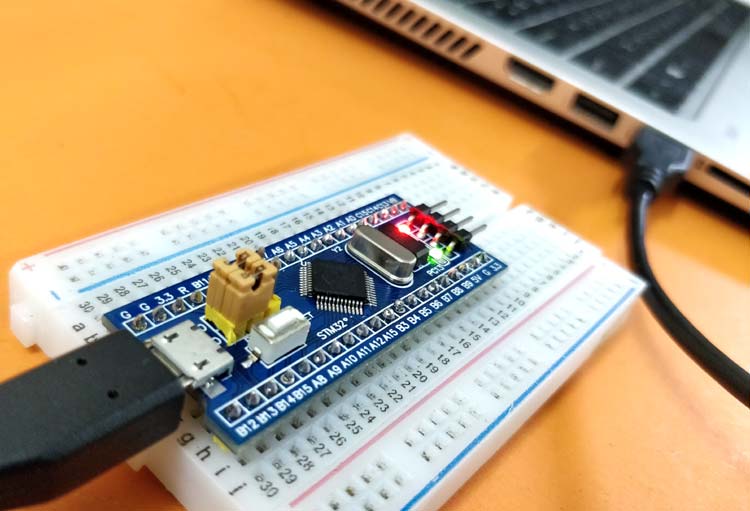
Instead, I started looking into STM32 devices. First I considered the STM32F103C8, which seems to be very popular. It has a 16 bit timer running at 72 MHz, so it’s capable of achieving the PWM rate. It features 2 SPIs with 18 Mbit/s and allows full-speed USB 2.0, which is supposed to reach 480 Mbit/s, much more than the 256 kBit/s I need. It’s dirt cheap too, at about €1. It looks like it could definitely do the job.
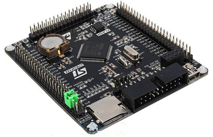
The thing is, I’m not entirely sure yet how many clock cycles my control loop will require. At 8 kHz, this 72Mhz clock can run 9000 cycles per iteration. That’s surely enough for a simple PID loop, but if I want to leave room for LQG or other more advanced techniques, spending €7 more for the beefier STM32F407VET6 might save me some headache down the road. I was recommended this particular board by Enzo Evers, who is working on similar projects, check out his work here.
This microcontroller comes with a bunch more timers too, supports virtual COM ports (which is supposed to be more convenient than regular serial, from what I’ve heard) and features a 168 MHz clock (and consequently, either a higher PWM frequency or higher resolution, which is nice too). Oh, and it has an SD card slot. It’s great value, speaking from my experience with it since the start of the project.
To flash my code to the microcontroller, I use an ST-Link v2. You can get a clone for around €1.50. It’s an USB-stick with pins that connect to the corresponding pins of the microcontroller, see this guide for how to wire it up. Warning: depending on where you got your ST-Link, the pins might be wired differently. I’d go with the pin order written on the device. For me, this was different than the order of the guide I was using, and it took me way too long to figure that out.
With the most important choice out of the way, that just leaves us the hardware for the motor control. At the moment, I decided to go for the L298N H-bridge, a popular DC motor driver that supports 24V and 1 A.
The thing is, if PWM (so, voltage) is the input to the printer, the input is not proportional to torque, which scales with current. Most systems I’ve worked with in my studies have current as input, I still need to look into if I want this, why, and if yes, how. That’s scheduled for part 4; I’ll update this post if I end up buying something extra. Any tips are welcome in the comments.
So for now, the last thing that remains is a 24V power supply. I ended up buying a Mean Well LRS-150-24.
Auxiliary parts
For the next part, setting up the real-time platform, I’ve found it very useful to toggle GPIO pins and read them out with a logic analyzer. I ended up buying this one for €5. And of course, I got a whole load of different cables.
In the next post, I’ll explain how the real-time control loop is set up.
With all the hardware selected, let’s start working on obtaining a real-time control loop. I’ll first describe how I set up the software, then go into how I configured the STM32 board and how to communicate with it, and lastly I’ll verify that everything is working as it should.
Preliminaries: software
STM32 microcontrollers can be conveniently configured using STM32CubeMX. You can install it from here. In this program you can easily configure the role of the pins and clocks, and it spits out a convenient code template for your IDE of choice. For the IDE, in which you write and compile C code and flash the program via the ST-link to the STM32, I chose Keil MDK-Arm, found here. To use the ST-Link v2, you’ll need this driver. You can update the filmware of the ST-Link using this utility program.
Some STM32 devices ship with an stm32duino bootloader, such that you can program it in the Arduino IDE. I did not want this, since I figured it would offer less control of the hardware timers and corresponding registers (but maybe it’s possible that way too). To get rid of it, you can erase the stm32 device via the ST-Link utility mentioned earlier.
STM32 board configuration
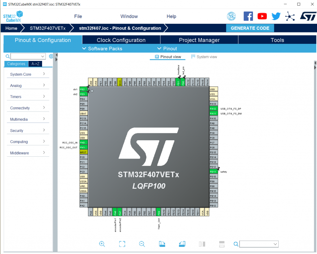
Once you’ve installed all these programs, open STM32CubeMX and start a new project. Select your STM32 board, in my case STM32F407VET6. You’ll be greeted with this screen:
except that I already configured some pins, and yours will be grey without label.
Timer configuration
Let’s start with the most important parts: the timers. One to drive the real-time loop, one to generate a PWM signal and one to keep the encoder count.
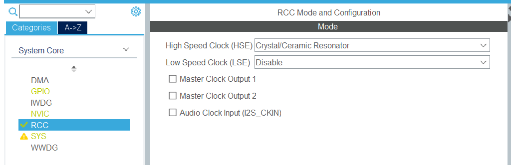
First, click “System Core” in the left tab and click RCC. Make sure the High Speed Clock (HSE) is set to the Crystal/Ceramic Resonator:
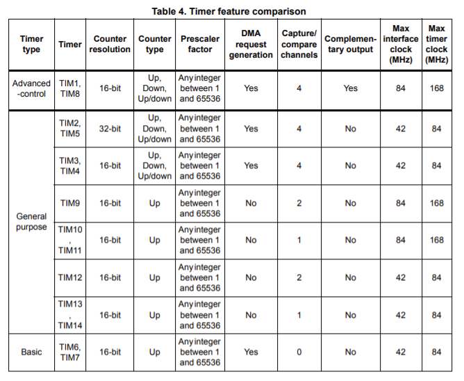
Then, we need to choose which timer to assign to which task. An overview of the timers is found in the datasheet:
Before moving on, let’s get into more detail about how to interpret these numbers. When configuring a timer, we can set the timer period T_clock, i.e., the number of counts that the timer will do until it will reset. This is at most 2^resolution in the third column. It will count with the frequency f_clock of the rightmost column.
So the frequency at which the timer resets is f_timer = f_clock / T_clock.
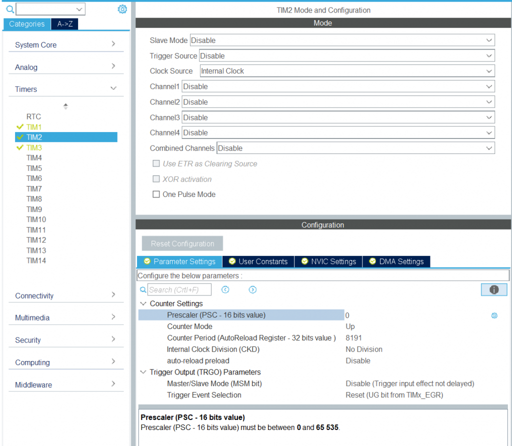
Timer for real-time loop
The timer driving the real-time loop needs to trigger an interrupt at at least 8 kHz, the counter resolution is not directly relevant here. Let’s pick TIM2 for this. Since it runs at 84 MHz, let’s choose a timer period T_clock = 2^13 (not that we’re limited to powers of 2, but I prefer this). This is leads to a sample frequency of 84e6 / 2^13 = 10.25 kHz, a little more than we need. In the Timers -> TIM2 menu in the sidebar, enter this:
Note that it takes T_clock - 1 = 8191. In the NVIC Settings tab, check the box so that it triggers a TIM2 Global Interrupt whenever the timer resets.
PWM timer
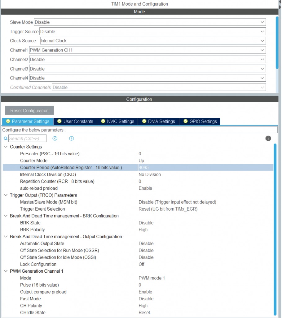
As mentioned in the previous post, the PWM timer is the most critical one. A higher counter resolution allows us a finer range of voltages we can apply, and the clock frequency needs to be over twice the sample frequency. For this reason, let’s pick TIM1 for the PWM timer.
If you’re PWM frequency is in the human hearing range, you can actually hear it squeaking while it’s running. While originally I set the requirement that the PWM frequency must be 2 times the sample frequency, I now doubled it to 41 kHz to get rid of the ~21 kHz sound. Since TIM1 runs at 168 MHz, this corresponds to a timer with a period of 2^12, since 168e6 / 2^12 = 41 kHz. This is exactly the minimum required resolution set in Part 1.
To configure this timer, go to TIM1 in the sidebar of STM32CubeMX and select the following options:
See this for more info on PWM on STM32 microcontrollers.
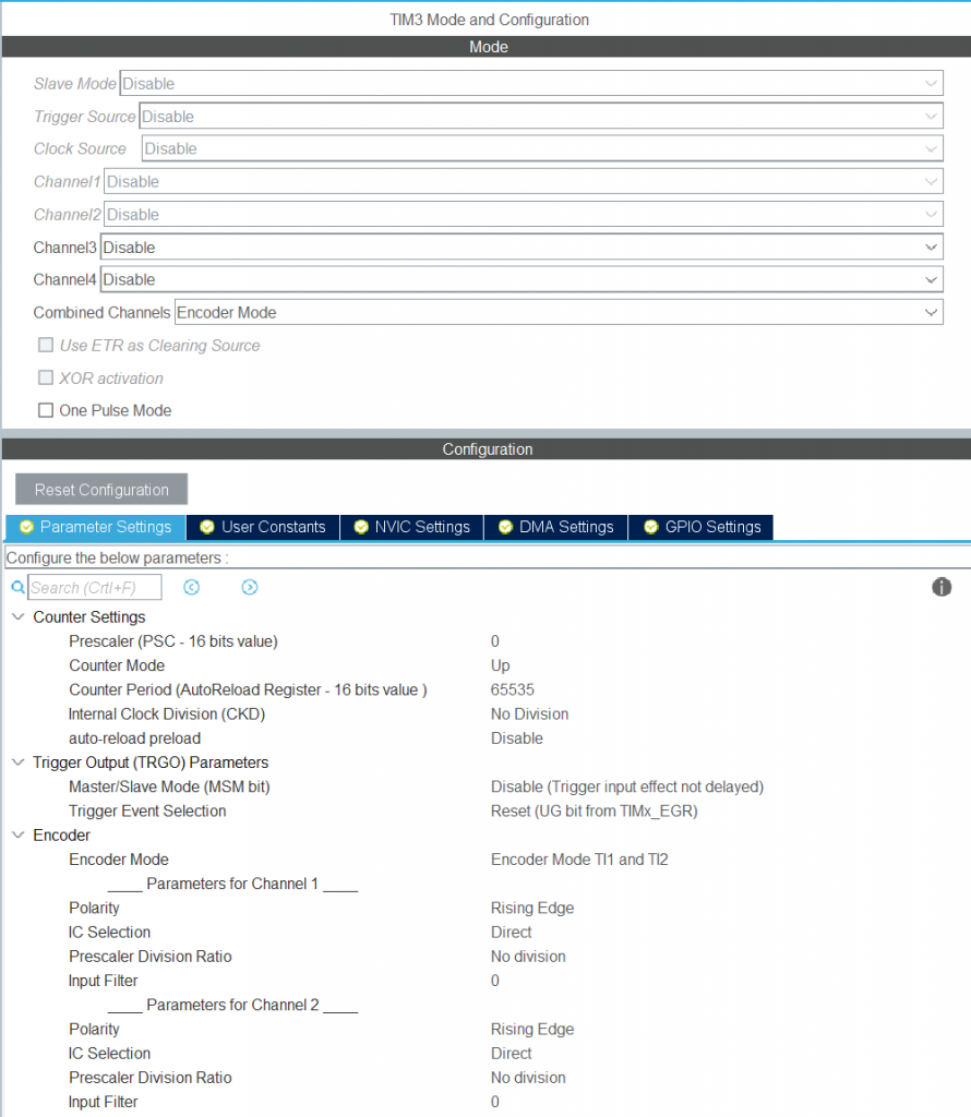
Encoder timer
The photo-interruptor can be interpreted as an encoder and set up by following this guide. I use TIM3 for it. The only difference is that I don’t use an input filter (haven’t read up on what it does, but I’ve been keeping it at 0 and it works fine. Want to keep things as simple as possible). Since our strip has about 8000 slits, a 16-bit resolution is sufficient, so we enter 2^16-1 for the timer period:
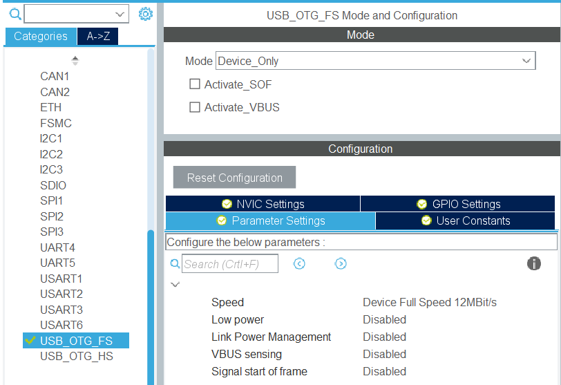
USB configuration
We’ll communicate with the STM32 over USB using a Virtual COM port. I’m not sure what guide I used at the time, but this one seems similar (but on the STM32F407VET6 you can use the on-board USB port). Go to Connectivity -> USB_OTG_FS and select the following:
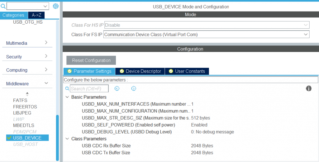
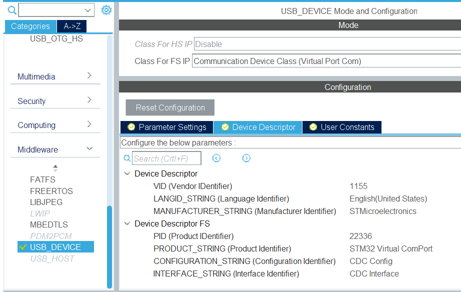
Also select Middleware -> USB_DEVICE:
GPIO configuration
Some pins will be assigned functions automatically based on the settings we’ve configured. However, by right clicking a pin on the STM32 microcontroller image on the right, you can select GPIO_Output and assign it a label. Do this for 2 pins such that we can control the direction of the DC motor, and one more so we can output a ‘heartbeat’ pulse every time we enter the control loop.
Writing the code
In the Project Manager tab on top, select MDK-ARM for the toolchain / IDE and then click Generate Code on the top right. Open the generated .uvprojx in Keil to find the template code.
Code for the real-time loop
In the template, some parts will be managed by CubeMX if you regenerate the code, and some parts are left to be programmed by the user. The latter parts are marked by “USER CODE BEGIN …” and “USER CODE END …”.
I’ll describe next how to set up the bare basics for the real-time loop. If enough people are interested, I’ll consider cleaning up my full code and sharing it on Github.
In “USER CODE BEGIN Includes”, include the following libraries:
This flag will be set by the interrupt handler. The main loop will execute when this flag is set, and then reset the flag. In “USER CODE BEGIN 1”, inside the main() function:
// Send N samples over USB per buffer
int N = 100;
// Number of bytes sent per sample
int len = 4;
// Initialize the buffer
uint8_t buf[len*N];
// Initialize the iteration counter for USB
int iter = 0;
int16_t encoderPos = 0;
// Set the maximum PWM value at 65% for testing
uint16_t max_pwm = 4096 * 0.65;
uint16_t u;
if (flag) {
    //Make sure an interrupt doesn't interfere with setting the variable
    __disable_irq();
    flag = 0;
    __enable_irq();

    HAL_GPIO_WritePin(heartbeat_GPIO_Port,heartbeat_Pin,1);
    encoderPos = (int16_t) TIM3->CNT;

    u = max_pwm; // For testing
    //Set the motor direction
    HAL_GPIO_WritePin(dir1_GPIO_Port,dir1_Pin,1);
    HAL_GPIO_WritePin(dir2_GPIO_Port,dir2_Pin,0);

    // Copy the encoder position and input voltage to the buffer
    memcpy(&buf[iter*len], (uint8_t *) &encoderPos, sizeof(int16_t));
    memcpy(&buf[iter*len+2], (uint8_t *) &u, sizeof(int16_t));

    if (iter==N-1) {
        iter = -1; // reset iter

        // Send the buffer over USB
        CDC_Transmit_FS(buf,len*N);
    }

    iter++;
    HAL_GPIO_WritePin(heartbeat_GPIO_Port,heartbeat_Pin,0);
}
Lastly, to let the interrupt of TIM2 set the flag, add this function to “USER CODE BEGIN 4”:
void HAL_TIM_PeriodElapsedCallback(TIM_HandleTypeDef *htim) {
	if (flag) {
		HAL_GPIO_TogglePin(led_pin_GPIO_Port,led_pin_Pin);
	}
	flag = true;
}
The LED now functions as a simple overrun detector.
With the code set up, you can compile the code in Keil with F7 and flash it to the board with F8. When it’s done downloading, don’t forget to press the reset button on the STM32 board to run the code.
Communication
To read the messages coming from the STM32, I use realterm. In the PORT tab, select the a sufficient Baud rate (921600 bits/s is more than enough for 2 int16_t variables at 10.25 kHz) and in the Port tab, select the virtual COM port of your device. For me, it’s “9 = \USBSER000”. Open the port and go to the Display tab to select int16. To record a measurement to a file for analysis, just enter a path in the Capture tab and press Start.
Validation
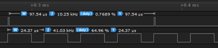
If we analyze the heartbeat pin and the PWM signal with the logic analyzer, we get:
As expected, we have 4 PWM cycles in one sample, and the sample frequency is 10.25 kHz, which is correct. Let’s take a closer look at the recorded heartbeat signals.
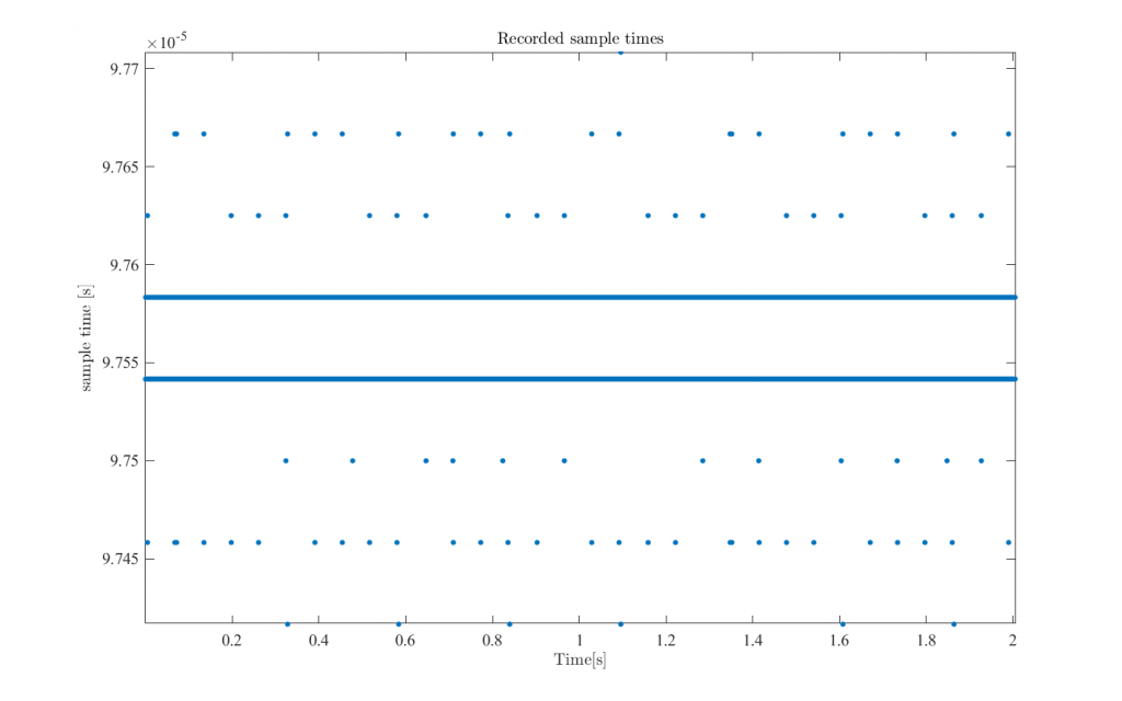
If we plot the difference between timestamps when the heartbeat signal becomes HIGH (let’s call this diff(tauvec)), we get a vector of all recorded sample frequencies. Plotted against time, this becomes:
Note that the desired sample time is 9.752 * 10-5 seconds, about 0.04% lower than the average measurement, but the difference is constant, so I’m fine with this. Next, notice that the recorded sample times are spaced with equal distance. Here is a histogram of diff(tauvec):
The two peaks at +-41.6667 ns must be the resolution of my logic analyzer. If the real sample time is not an exact multiple of the resolution, it will regularly snap to the next resolution step. This would also explain the regular pattern in the blue plot above.
For these reasons, I’m willing to call this control loop hard real-time, and assume that the sample time is constant at all time. Of course, as I expand the code executed inside the control loop, I will monitor the overrun detection.
If there are any questions, or if you disagree with any claim, feel free to let me know in the comments. I hope it’s at least useful to someone trying to set up their project 🙂
In the next post, I describe how I did an FRF measurement of the printer and designed a simple controller.
In the last post, I set up the basics of the real-time platform, such that it’s possible to run a control loop and transmit data to and from my PC over USB. I have since expanded this platform to work together nicely with Matlab: I have a Matlab function to send signals (e.g., reference or feedforward signals) to the STM32, which copies it to the right array to be used in the control loop.
With this, I can finally start with the control engineering phase. In this post, I’ll explain how I measured a Frequency Response Function (FRF) in closed loop, fit a transfer function and how I designed a simple feedback controller. This is all done with the end-goal in mind: the implementation of Iterative Learning Control (ILC) using a real-time platform worth less than €10 (not counting the power electronics).
I assume quite some prerequisite knowledge of control engineering here. If you have trouble understanding something after reading the references mentioned in the first post, feel free to ask a specific question in the comments.
FRF measurement
There is a lot of friction on this printer. To get the carriage to move at all, I need a PWM duty-cycle (which scales with voltage) of 65%, using my 24V power supply. This leads to important limitations for both the FRF measurement and controller design.
Static friction is non-linear. However, we want to make use of linear control theory, so we need a linear (approximate) model. To this end, we measure the FRF in closed loop in such a way that the carriage is moving most of the time – whenever it’s moving, it’s unaffected by static friction. Measuring in closed-loop also helps prevent the carriage from slamming into the side of the frame, waking up my dog.
A closed-loop FRF measurement does pose a challenge: we need a feedback controller, even before we have a model. The nice thing about this voltage-controlled setup is that the bode plot of the system G(s) starts with a -1 slope at low frequencies, only to decrease to -2 after the pole caused by the motor inductance. Consequently, constant input voltage leads to constant velocity, because of the back-emf of the motor. If the input were current, the system would start with a -2 slope. Since we start with a -1 slope, the Nyquist plot of the open loop, with a proportional controller C(s) = k for some small k, is stable:
Rough Nyquist sketch of a possible G(s) when starting with a -1 slope: closed-loop stability may be achieved with a small gain.
So by starting with a small gain, the closed loop will at least be stable and an FRF measurement is possible.
I opted for the three-point method (see the last part of ‘FRF estimation in closed-loop systems’ here): inject a voltage d to the system in closed-loop, measure both the error e and control effort u = d+C e, compute the sensitivity and process sensitivity and infer the system G(s) from these. As opposed to the two-point method, this doesn’t require knowledge of the controller. Of course, I implement the controller myself but since I was changing it a lot, it was convenient not having to have to keep the Matlab code consistent with the C code running on the microcontroller.
For the disturbance I chose a square wave with an amplitude of 65% duty cycle plus zero-mean white noise. With a reference of zero and a proportional controller C(s)=10 (which was found by starting with a very small gain and increasing it slightly between experiments), this leads to a back-and-forth motion around the center:
Control effort u (feedback+feedforward) and error e during the first two seconds of the FRF measurement. The total measurement took about 2 minutes.
The white noise was generated on the STM32 using this code, this way I don’t need to send huge arrays of random numbers to the microcontroller.
The FRF measurement. In closed-loop with r=0, the carriage is always ‘pulled’ towards the center.
The resulting two minute FRF of the system G, using Hann windowing with a 1/3 second window size, looks like this:
Bode plot of the FRF of the printer. You can clearly see the resonance and anti-resonance around 300 Hz.
Below 200 Hz the coherence is really not that great so the FRF should be taken with a large grain of salt:
Coherence between u and d (left), e and d (right)
It’s not perfect, but for the purpose of having a decent model for ILC, we can work with this.
Parametric model
For ILC we need a parametric model of the process sensitivity PS(s) = P(s) / (1+P(s) C(s)). To that end I made a fit of G with one integrator that looks like this:
Bode plot of the FRF and the fit.
It’s not perfect, but as I’ll show in a future post, it’s enough to lead to great results using ILC.
Controller design
The end-goal of this blog series is to implement ILC on the printer. With ILC, as I’ll explain more in a later post, a feedforward signal for a single task is learned iteratively. However, we also want a feedback controller, for e.g. attenuation of disturbances.
Controller design for this system is cumbersome, because the feedforward voltage required to get the printer to move at all is 65% of the maximum voltage. This leaves 35% for feedback. As it turned out, with any kind of pole in the controller close to the unit disc, the feedback signal would saturate in no time. Saturation, in which a duty cycle of >100% is forced back to 100% is a non-linear action, so all linear control theory can be thrown out the window. Often times, when this happened, the feedback signal would jump between 100% and -100% every sample, leading to me frantically rushing to pull the cable out.
As mentioned before, for a low bandwidth controller we really don’t need phase lead, because G starts with a -1 slope at low frequencies. I also don’t really need an integrator, because with (parallel) ILC this could lead to the ILC signal and the feedforward signal working against each other. For that reason, I went with the low bandwidth controller C(s)=10, such that the bandwidth lies around 17 Hz (very roughly, mind that the FRF isn’t perfect at low frequencies) and the Nyquist plot of the open loop looks like this:
Nyquist plot of L=CG, with C(s)=10. Mind that the quality of the FRF is not great at low frequencies, but this indicates that we very well may have closed-loop stability, assuming G has no poles in the open right half plane. Experiments confirmed this.
Since it proved that this controller with ILC led to performance that I was happy with, I didn’t go further than this. I’m aware that there are techniques that deal with saturation of the feedback signal, but I didn’t feel they were in the scope of this project.
In the next post, I’ll show how I successfully implemented Iterative Learning Control with this model and controller, leading to an error in the order of 0.1 mm (a few times the encoder resolution) during constant velocity. If you don’t want to miss it, make sure to subscribe to the e-mail notifications in the sidebar 🙂
In the previous post, I designed a feedback controller and obtained a model of the printer. With that, all the ingredients are in place to implement Iterative Learning Control (ILC).
ILC is a learning method to learn a feedforward signal to perform a certain task iteratively. It requires a model of the system, which need not be perfect, and it requires the task (reference) to be the same every time. Moreover, there exist elegant conditions for monotonic convergence that make the design procedure relatively straightforward. If you’re unfamiliar with ILC, I recommend starting with, for example, this 2-page summary before reading on. A lot more references, e.g., for dealing with task flexibility or describing lifted ILC, are included here. In this post, I will apply frequency-domain ILC.
Goal
The aim is to track the following third-order reference with the least positioning error possible:
Since the application is a printer, the constant velocity part is deemed most important.
Learning filter design
The ideal learning filter L(z) is the inverse of the process sensitivity (in this post, L(z) does not represent the open-loop!). Since the process sensitivity is causal, i.e., the discrete-time system has more poles than zeros, the ideal learning filter is non-causal. Consequently, the feedforward signal at time t depends on the error at some time t+a in the future. Moreover, if PS(z) has non-minimum phase zeros, which my model does, 1/PS(z) has poles outside the unit disc.
To simulate this, I use stable inversion, in which the unstable part of L(z) is split from the stable part and simulated backward in time – a ball rolling off the peak of a hill is an unstable response, but not if you play it backward in time! There’s more info on this in the links shown before.
Without a robustness filter, ILC would converge monotonically if |1-GS(z) L(z)|<1 for all frequencies. Let’s evaluate:
|1-GS L| for both the FRF and the model. Even if the FRF were perfect (which it isn’t), with this parametric model of G we would require a robustness filter Q, because the plot exceeds 0 dB.
Right now, the condition for monotonic convergence is not met. We need a robustness filter Q for that.
Robustness filter design
With a robustness filter Q, the criterium for monotonic convergence becomes |Q’ Q (1-GSL)|<1 for all frequencies, where ‘ denotes the conjugate transpose. With Q a first-order lowpass filter with a cutoff frequency of 80 Hz, we get:
|Q’ Q (1-GSL)|. Since 0 dB is not exceeded, we would have monotonic convergence if the FRF were perfect.
The filter is quite conservative, but since the FRF is imperfect, this gives us some margin for error. The price paid for this is that the final error of ILC, after convergence, will be higher: we don’t learn nearly as much at frequencies above 80 Hz now. Still, as shown below, this is enough to achieve some nice results.
Results
Let’s start with the results before ILC. Using the feedback controller of the previous post and a feedforward signal f=0.65 U sign(v), where U is the maximum voltage and v is the velocity of the reference profile, we get:
Results without ILC. With an encoder resolution of about 0.035 mm/count, 50 counts corresponds to 1.7 mm.
When implementing these L and Q filters, using a learning rate of α=0.3 (see the references mentioned, this is for attenuation of trial-variant disturbances), this is what happens:
Error over iterations with ILC. Only every 4th trial is plotted for clarity.
We have nice convergence:
2-norm of the error over iterations.
At the final trial, the performance is much better than what we started with, a factor 8 smaller in the 2-norm and a factor 3.6 smaller in the infinity-norm:
Performance after 20 trials of ILC. During constant velocity, the peak error is 3 counts: only 0.11 mm.
I’m very happy with these results; it really shows the strength of ILC: with a simple feedback controller and a low-quality model, the performance is improved significantly in 20 trials. And that on a ~€6 microcontroller!
Recommendations
What if you wanted to decrease the error even further?
Analyzing the amplitude spectrum of the error profile after 20 trials of ILC, ignoring the samples where the reference is zero, we have:
Amplitude spectrum of the error after ILC, ignoring the samples where the reference is zero.
The oscillating behavior in the error is clearly seen as a peak in the spectrum at 19 Hz. Hence, a good place to start could be to either (i) increase the model quality at 19 Hz, such that that the learning filter better represents the real system at this frequency and learns to reduce the error here, or (ii) reduce this error with feedback, using an inverse notch filter at 19 Hz. Either way, I’m happy with the results as they are now, but there’s plenty of steps forwards.
Conclusion
Do you need a setup worth thousands of euros to play around with learning control techniques? As it turns out, a €6 microcontroller is enough. While I have access to Matlab, everything may as well have been done using Python or any other language since the communication to and from the microcontroller is all done using the standard Serial protocol.
I plan to make one more post in this series explaining what I learned about the practical side of control during this project. After that, I’m applying this real-time framework to other projects, so if you don’t want to miss that, subscribe to e-mail notifications in the sidebar!
In the previous post, the end goal of this project was reached: the implementation of Iterative Learning Control using less than €10 worth of hardware.
In this post, I’ll explain what I’ve learned on the implementation aspects of control during this project. A lot of these things are probably elementary if you have a background in electrical engineering, but as a control engineer with a mechanical engineering background, I had to figure these things out as I went. Hopefully, this post can help people with a similar background to learn more about the practical side of things. Disclaimer: I’m no expert by any means when it concerns electronics, so if I’m wrong about something, I’d love to be corrected in the comments or through the contact form.
First, I’ll cover what I learned about the implications of using PWM in a control loop. Second, I’ll explain what I learned about the difference between current control and voltage control. Lastly, I’ll give a more general evaluation of the project and point to some possible improvements.
What it means to use PWM in a control loop
From my university classes in the Mechanical Engineering department, I’m used to the convenient assumption that we can apply any input u(t) to a system. If only things were so simple in practice.
I learned that when working with microcontrollers, there are two main ways to send an analog signal: 1) using a DAC, and 2) using PWM. These two methods have a few things in common:
The signal coming from the microcontroller is <5V, so some kind of amplifier is needed in between the microcontroller and the DC motor.
The resolution of the analog signal is limited to 2n possible values of u(t), where n is a number of bits.
As far as I’m aware, a major advantage of switched methods such as PWM is increased efficiency. Since I got an L298N motor driver board early on, which works with PWM, I didn’t look much further into DACs. Therefore, from here on, I’ll focus on PWM.
Using PWM to generate analog signals
As it turns out, PWM can be used to ’emulate’ a DAC: we compute a desired u(t) on the microcontroller, set a duty-cycle to generate a high-low pulse signal (i.e. we encode our desired input to PWM), and by low-pass filtering this signal, an analog signal is obtained (it is decoded again).
But how do we know the ‘decoded’ signal matches our original desired signal u(t)? Is this operation of encoding and decoding even linear? Since I wanted to use linear control theory, this is a critical requirement. Eventually, I learned that indeed, knowing whether the analog signal matches the original desired u(t) is not at all trivial.
What can go wrong with PWM? Why even worry?
This page of Open Music Labs nicely explains it. In short, when the carrier frequency of PWM is insufficiently high with respect to the sampling frequency, we get harmonic distortion of the real signal u(t) with respect to the desired signal u(t). Also, recall from Part 3 that if we want twice as much resolution (possible values that u(t) can take), we need to halve the carrier frequency.
Now, there are some very interesting techniques to get rid of PWM distortion completely using sophisticated nonlinear computation of the duty cycle, and it would be very interesting to see the difference that these methods make in practice, but this just goes beyond the scope of my project. Let’s keep the scope limited to selecting the right carrier frequency.
On the STM32F407VET6, there is a 16-bit timer running at 168 MHz, so if we want a 12-bit resolution, we have a carrier frequency of at most 41 kHz. We want the sample time of the control loop to be sufficiently high because discrete-time delays can limit the achievable performance of the closed-loop. From the page on Open Music Labs, we find that if we sample too fast, we can end up with quite some harmonic distortion of the signal. This is why I’d been worried about this in the first place.
Trade-off between sample time, resolution and PWM distortion
In this project, the open-loop bandwidth was around 20 Hz, and phase lag caused by discrete-time delays was not the limiting factor. Therefore, I decided to lower the sample time to 2 kHz and choose a carrier frequency that was a factor 8 higher. I used a continuous-time Simulink model with a PWM block to verify that with these numbers, the PWM distortion was acceptable (it really wasn’t when the carrier frequency was around 2 times higher). This allowed for a 14-bit resolution. It might have been better to lower the resolution in return for even more carrier frequency, but at this point, I realized something that largely ended all my worries about making the right choices with PWM.
Why I probably didn’t need to worry that much about PWM distortion anyway
Let’s view the harmonic distortion on u(t) caused by PWM as a disturbance d(t), i.e., input noise. The same holds for quantization effects; we don’t have an infinitely high resolution, so let’s say that the mismatch with the desired u(t) is also lumped into d(t).
Both of these input disturbances are likely high-frequent, varying roughly at the time scale of the sample time but not around the bandwidth of ~20 Hz. In closed-loop, the transfer from d(t) to the error e(t) is the process sensitivity, i.e., PS(z) = P(z) / (1+C(z)P(z)). At high frequencies, the process sensitivity approximately equals the plant P(z), which has a negative slope at high frequencies.
So it might be a good idea to be aware of the fact that the carrier frequency is not too low w.r.t. the sample time, and you don’t want your input resolution to be too low either (I think 12 bit is used a lot in practice), but if the choice is imperfect, its contribution to the error will likely be marginal because it is filtered with the process sensitivity. Output noise on y(t), on the other hand, is transferred to the error through the complementary sensitivity T(z) = P(z) C(z) / (1+C(z) P(z)), which approximately equals P(z)C(z) at high frequencies. With high controller gain, output noise is therefore much more likely to be problematic than input noise.
Nevertheless, it was very interesting to learn more about this, and at least I feel like I know much more about different sources of input noise now.
On voltage control vs. current control
When modeling motion systems, it can be convenient to view the torque T(t) as an input to the system. In DC motors, torque is proportional to the current. However, the output of our microcontroller is a voltage. So do we just use voltage as an input? Or do we need to do something more?
Consequences of using voltage as an input
From this model of a DC motor, we have the following transfer function:
If we measure position instead of velocity, an integrator is added to the transfer function. The resulting 3rd order system then has one integrator and two poles, the location of which depends on motor inductance, electric resistance, viscous friction, the motor constant, and inertia. With only one integrator, a constant input (voltage) leads to a constant velocity of the printhead.
Suppose we want to control the torque of the motor directly – for example, because we want to use basis functions feedforward based on the differential equations of the dynamics (where input is torque). What do we do then?
Using cascaded control to effectively have current be the input
With feedback, you can change the location of the poles. With cascaded control (see e.g. Multivariable feedback control by Skögestad), you could change the printer system from being an open-loop system P(s) to being a closed-loop system P(s)C(s)/(1+P(s)C(s). The reference to this closed-loop system is desired current (expressed physically by a voltage) and the output is the measured current.
From the link at the beginning of this section, it can be derived that the transfer from voltage to voltage to current resembles a low-pass filter. Hence, a high bandwidth can be reached easily using a simple PI-controller. Since the closed-loop transfer is approximately one below the bandwidth, this means that up until this high bandwidth, you can essentially control the torque by changing the reference voltage (which represents desired current now).
I worked this out in a simple Matlab script to demonstrate how this could work as an example. How to actually implement this current controller is a topic for another project. In this printer project, I just used the voltage as an input, which is perfectly possible too.
Evaluation & conclusions
This project taught me a lot about discrete-time control, real-time systems, and electronics. I find that doing such a large project is a great way to learn how to apply theory in real systems.
So, as it turns out, it’s perfectly possible to implement advanced motion control techniques even with cheap hardware. It is more cumbersome to write C than to drag and drop Matlab blocks, but at such a low price it’s great.
I already have some ideas for the next project, which will likely involve MIMO control, repetitive control, or both. Subscribe to the newsletter in the sidebar to get a notification when I write a new post and feel free to leave questions in the comments.


![$$ P(s) = \frac {\dot{\Theta}(s)}{V(s)} = \frac{K}{(Js + b)(Ls + R) + K^2} \qquad [ \frac{rad/sec}{V}] $$](https://ctms.engin.umich.edu/CTMS/Content/MotorSpeed/System/Modeling/html/MotorSpeed_SystemModeling_eq07187872419275675603.png)